In this series of articles, all of the regression discussions to date have assumed that the replicate preparations of a given concentration have been exact. Two of the key diagnostics (i.e., modeling of response standard deviation [SD] and the use of the lack-of-fit [LOF] test) require such duplication. However, in some analytical methods, this exactness is not possible. (The authors will now “fess up”! In reality, the ppt-level chloride and nitrite examples, which have been used repeatedly in past articles, did not involve exact replicates. To avoid contamination, standards at these low levels are prepared strictly by pouring [no use of pipets], so the desired final volume is never actually achieved. Within this American Laboratory column, the concentrations were rounded to the target values, which were “good enough” for a first approximation. The authors considered that this deviation from reality was minor and simplified the main discussions about regression diagnostics, etc.) How does the analyst proceed when only inexact replicates are available? This article will detail the regression-analysis steps for such cases.
At the outset, a few definitions are in order:
- Actual response: the raw response that was generated by the instrument
- Actual concentration: the true concentration of the standard, as calculated from the masses that were recorded accurately during the preparation process
- Target concentration: the desired concentration for a particular standard
- Group: a specific target concentration
- Mean concentration: the mean (or average) of the actual concentrations within a particular group; a statistic that is representative of a group’s actual concentration
- Scaled response: a raw response that has been scaled to its respective mean concentration.
In general, the goal is to devise a protocol that will scale response data to the mean for each group of concentrations. Such scaled and mean values will provide adequate replicates for use in SD modeling and LOF testing. However, for this procedure to be statistically sound, there should be a minimum of three observations per group (and preferably five or more). Details are as follows.
Step 1: Check responses for trends within each group of concentrations
This initial step involves grouping the data by the target concentrations. Within each group, plot the actual response versus the actual concentration, and regress a straight line (SL) with ordinary-least-squares (OLS) fitting. For each concentration’s plot, a p-value (for the slope) of ≥0.01 means that the slope is not significant; thus there is no statistically significant trend to the data. If the p-value is below this threshold, then the data do trend with concentration, and the analyst should think carefully before proceeding with regression analysis; the range of the actual concentrations within each group is probably too large to be considered a unit.
Step 2: Calculate the mean concentration for each target-concentration group
This quick procedure generates a value that represents the group, and can be used to model the SD and perform the LOF test.
Step 3: Scale the actual responses to each mean
Plot the actual responses versus the actual concentrations. Regress an SL with OLS fitting. The desired statistic is the slope of the line. (This model and fitting technique may or may not be appropriate in the end. However, it is an adequate approximation for purposes of determining the slope of the regression line.) Such a slope can be used to scale each actual response to its respective mean.
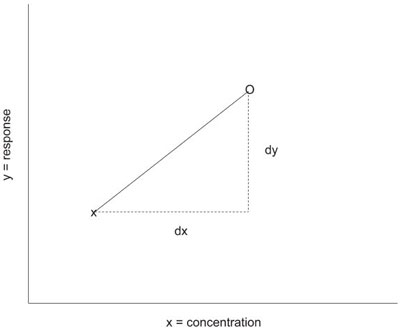
Figure 1 - In this diagram, the original data point is “x” and the scaled data point is “o.” The slope of the line connecting the two points is dy divided by dx.
Recall that in regression:
slope = dy/dx, or
dy = slope * dx
In this case,
dx = (mean concentration) – (actual concentration)
Once dy has been calculated, the actual responses are scaled:
scaled response = actual response + dy
See Figure 1 for an illustration of this process.
Now that both mean concentrations and scaled responses are available, exact-concentration data are at hand for SD and LOF testing.
Step 4: Model the standard deviation
For each mean concentration, calculate the SD of the associated scaled responses. Plot these SDs versus the mean concentrations. Regress an SL with OLS fitting. If the p-value of the slope is ≤0.01, then the SDs trend with concentration, and weighted least squares (WLS) is needed for the fitting technique. If weights are needed, the equation for this regression line is used to generate weights (see Part 8, American Laboratory, Nov 2003, for details on this calculation).
Technically, if WLS is the appropriate fitting technique, then Step 3 should be repeated, using the weights from Step 4 to regress the SL and scale the responses. These new scaled data are then used to iterate Step 4. If the differences between the original and new weights are deemed insignificant, then the protocol can continue to the next step.
Step 5: Test the proposed model for the actual data
Once the fitting technique has been determined and, if necessary, a weight formula has been established, the actual responses and concentrations can be regressed versus each other to test the proposed model. The residual pattern for this plot can be evaluated to assess its randomness, and a decision on model adequacy can be made on this basis.
Step 6: Perform an LOF test, using the scaled responses and mean concentrations
A more formal assessment of model adequacy can be made by plotting the scaled responses versus the mean concentrations. Since this plot involves exact replicates (i.e., the mean concentrations) for each concentration group, the traditional LOF test can be used after the proposed model has been fitted using the appropriate fitting technique. If the p-value for this test is ≥0.05, then the model is adequate. If the test fails, then iterate starting with Step 5 until an appropriate model is found. Once that goal has been reached, the prediction interval should be plotted (on the final graph from Step 5), and its width evaluated to decide if the uncertainty is low enough for the problem at hand.
The next installment will work through example data to illustrate the above protocol.
Mr. Coleman is an Applied Statistician, Alcoa Technical Center, MST-C, 100 Technical Dr., Alcoa Center, PA 15069, U.S.A.; e-mail: [email protected]. Ms. Vanatta is an Analytical Chemist, Air Liquide-Balazs™ Analytical Services, 13546 N. Central Expressway, Dallas, TX 75243-1108, U.S.A.; tel.: 972-995-7541; fax: 972-995-3204; e-mail: [email protected].