In analytical chemistry, simple linear regression is often used to perform calibration or recovery activities. The process has two basic steps and begins with designing a study [i.e., selecting: 1) the concentrations and 2) the number of replicates to be analyzed]. Once the data have been collected, step two involves determining a fitting-technique-and-model combination that is adequate; the result is a mathematical expression that relates the responses to the concentrations, and provides a means for estimating analyte levels in samples.
The previous article (Part 46, American Laboratory, Feb 2012) ended with a brief review of a statistically sound approach to regression diagnostics. This article will look at some regression practices that are often adopted because they are easy to effect, but which are risky in the statistics world. Even though some of the subtopics have been addressed previously (at least briefly), they are included here for completeness. The first unwise practice involves the direction in which the data are analyzed. Regressing x on y is tempting for calibration, since the ultimate use of the curve is to determine a sample’s concentration (x) once a response (y) has been obtained from the instrument. However, one of the basic assumptions in simple linear regression is that the x-values are true and the y-values have uncertainty. Violating this fundamental will lead to noisy coefficients in the regression equation and compromise future results. Always regress y on x!
Study design
One design shortcut involves analyzing only one non-zero standard. To generate a regression curve for calibration or recovery purposes, a second concentration must be used; by default, that level is zero. With such a design, the user is assuming that: 1) there is never a measurable response for blanks, 2) response standard deviations do not trend throughout the range, and 3) there is no curvature in the data. It is not uncommon for at least one of these assumptions to be untrue. Additional comments are warranted on the inclusion of “hard” zeros in a set of calibration or recovery data. Even if a blank does not produce a response from the instrument, it is unwise to enter a zero as the y-value. Zero has no variation, yet how many zeros are entered will influence the regression line, at least to some extent. The best policy is to leave the response cell blank if the instrument does not generate a measurable signal. It also is never wise to force a curve through zero; the data and the regression process should be allowed to determine where the y-intercept should be.
If replicate data are collected using the single prepared standard, a standard deviation can be calculated. However, this statistic is not helpful in this situation; standard-deviation modeling requires multiple levels, along with replicates at each x-value.
A second unwise design is analyzing multiple concentrations of standards, but collecting no replicates. Standard-deviation modeling again is impossible. Detecting true curvature cannot be accomplished, either. Even if the points appear to lie in a curve, there is no way of knowing if the pattern actually represents the overall data set; the responses may be quite noisy and the current plot is simply “the luck of the draw” from an otherwise linear data set.
With both of the above designs, there are too few degrees of freedom to allow an adequate assessment of the data’s behavior. Also, it is not possible to generate a truly representative prediction interval, thereby precluding a sound assessment of the uncertainty associated with the analytical method.
Fitting technique
Another area where unwise procedures occur is fitting-technique selection. Many years ago (especially when instrumental software was not very sophisticated), it was typical to use ordinary least squares (OLS) with every data set. Currently, the coin seems to have been flipped, meaning that weighted least squares (WLS) is employed by default. Neither absolute is appropriate. Enough data should be collected to model the standard deviation (s) of the responses (y), as a function of concentration (x), so that an informed choice can be made.
Within the world of WLS, the recommended procedure for generating weights employs the formula for the modeled standard deviation. However, several shortcuts are available for calculating the weights, once replicates are available at each concentration. Options include the following:
a) 1/x
b) 1/x2
c) 1/y
d) 1/y2
e) 1/s
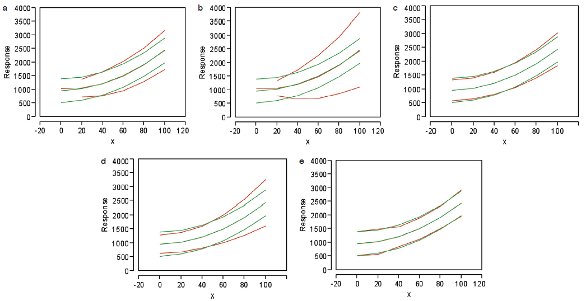 Figure 1 - A set of simulated data, plotted (in red) using various shortcut formulas for the weight. Also plotted (in green) is the case where the weight is based on the modeled standard deviation. The shortcut formulas are: a) (1/
x
), b) (1/x
2), c) (1/y
mean), d) (1/y
2mean), and e) (1/s
). In each set of curves, the identities from top to bottom are: upper prediction interval, regression line, and lower prediction interval.Using one of the above formulas may result in highly unrepresentative prediction intervals. In addition, any of the first four options presents an intractable problem when the divisor equals zero, since (1 ÷ 0) equals infinity. Furthermore, if one of the y-containing options is used, the y-values will have to be averaged first; otherwise, a different weight will be applied to each data point and the prediction interval will be quite jagged.
To illustrate the difficulties that can arise, consider the simulated raw data that were used in Part 45 (American Laboratory, Nov/Dec 2011); the standard deviation of the responses does not trend with concentration (i.e., OLS is appropriate) and a quadratic model is adequate. However, for purposes of discussion, assume that laboratory procedures dictate that WLS always be used.
What are the results of choosing each of the previously discussed formulas for the weights? The plots in Figure 1 show the outcomes. In each case, use of one of the shortcut formulas has been graphed (in red) along with the use of the modeled standard deviation (in green).
The regression line itself is not affected much by the choice of weight, although such an occurrence is not a given for every data set. The shape of the prediction interval is a different matter. In this example, the most dramatic contrasts (between shortcut and modeled weights) occur when an x-term or the y-squared term is involved. Other data sets may give other outcomes; however, the user cannot not know a priori how the various weight formulas will affect the prediction interval.
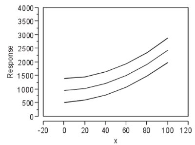
Figure 2 - Plot analogous to the ones in Figure 1. However, here, the curves generated via OLS are overlaid with the lines created using the weight based on modeled standard deviation. Both sets are plotted in black.
By contrast, see Figure 2, which shows the OLS fitting along with the modeled-s version of WLS. Since this data set can be fitted adequately using OLS, it is not surprising that the two plots overlay virtually exactly when the weight is generated in a statistically sound manner. Again, though, this occurrence is not a vote for always using modeled-s WLS; let the data “speak” for themselves to determine the adequate fitting technique.
Model selection
In the arena of model selection, it may be tempting to simplify life and decide that the choice will always be a straight line or always a quadratic model. Neither decision is wise; indeed, throughout this series, a variety of data-behavior situations have been encountered. Even for the same analyte, response behavior cannot be assumed to be consistent from one application to the next.
Two other models that are implemented occasionally are: 1) percent peak area and 2) point-to-point. The first option is often employed if no standard is available for the analyte. Whenever this technique is used, it should be made clear to everyone involved that results are not based on a typical calibration curve, and that uncertainty estimates are virtually unachievable.
Point-to-point calibration is easy to effect, but is not wise. An objective of fitting data with a model is to describe the underlying behavior as realistically as possible. Point-to-point connections depend on the concentrations selected, necessitate the use of the mean response at each concentration, and do not provide a plausible estimate of how the data are behaving.
Take-home message
In the end, the recommendation remains the same: Design the study carefully and diagnose the data using the sound statistical diagnostics that have been detailed in previous articles.
The next installment will deal with relative standard deviations (RSDs), another concept whose use involves risks, including pitfalls in the arena of data modeling.
David Coleman is an Applied Statistician, and Lynn Vanatta is an Analytical Chemist; e-mail: [email protected].