Statistics in the Laboratory: Pooling

In statistics, “pooling” describes the practice of gathering together small sets of data that are assumed to have the same value of a characteristic (e.g., a mean) and using the combined larger set (the “pool”) to obtain a more precise estimate of that characteristic. In medicine, for example, a statistical “meta analysis” pools the results of many clinical studies to try to find a deeper truth that might not be revealed consistently in each of the individual studies.

In this column, we’ll see how pooling variances can work to the advantage of analytical chemists and others who carry out routine measurements. When properly applied, it can save a lot of money.

Every discipline has core concepts. In chemistry, Avogadro’s constant is a core concept—we couldn’t do much quantitative chemistry without it. In statistics, the variance is a core concept—we couldn’t do much quantitative statistics without it.

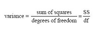
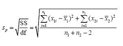
The variance s² is defined as a sum of squares (SS) divided by a degrees of freedom (df):

An estimated standard deviations is the square root of an estimated variance. Thus, the following equalities hold:

.

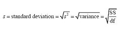As an example, the familiar equation for the estimated standard deviation of n data points about their mean x^- is:

where the Greek capital letter sigma (Σ) is the summation operator, and its index i indicates the measurement number from 1 to n. The numerator under the square root sign is clearly a sum of squared deviations of the individual data points about their mean, and the denominator is a degrees of freedom. Because one degree of freedom has been used to calculate the mean, only n – 1 of the deviations are independent. (And no, you can’t approximate the denominator as n if you have 30 or more data points—it’s always n – 1 for the kind of measurements you make. I don’t know how such misinformation gets into the literature. Why would you want to use an approximation, anyway, when you can do it correctly just as easily?)

So much for the basics. Figure 1 depicts a system that is used for making routine measurements. Samples 1 and 2 are physical (tangible) materials that are submitted for measurement. The numerical results (the intangible statistical samples) are shown as sets of circles, green for Sample 1 and blue for Sample 2. The numerical results and their means are shown on a measurement axis. The vertical dimension in this lower part of the figure has no meaning—the information is simply spread out upward.

Figure 1 – Application of a routine measurement method. In the upper part of the figure, Sample 1 and Sample 2 are physical samples of material that are submitted to the measurement process. The numerical results (the statistical samples) are depicted by sets of three circles, green for Sample 1 and blue for Sample 2. In the lower figure, the numerical results and their means are shown on a measurement axis; the vertical dimension has no meaning—it’s just a convenient place to spread out the information.

Let me step back a moment and emphasize something in the last paragraph. Chemists use the word “sample” to indicate a physical material. We all know what a sample is. We can touch it. In contrast, statisticians use the word “sample” to indicate a small subset of the results we might have obtained if we lived long enough (i.e., their sample is a subset of their conceptually infinite population). We can’t touch their sample. So, when a chemist and a statistician are having a conversation and using the word “sample,” it isn’t unusual to have each of them nodding their heads in agreement when, in fact, they have no clue what the other person is talking about. You have to be careful about this. There are a lot of words we have in common, but our meanings are different. It’s always a good idea to have the other side define their terms (and you define yours) if you suspect you might be having this problem.

Many measurement laboratories make multiple measurements on each sample that is submitted. These are called replicate measurements—they are repeated measurements of the same thing. In Figure 1, each sample is measured three times—there are three replicate results for each sample.

No one is surprised by this. Everyone seems to make replicate measurements. But why do we do this? I think there are three answers: 1) everyone else does it; 2) statisticians like big n; and 3) undergraduate quantitative analysis courses imply that you need to report a mean and a standard deviation for each physical sample submitted for analysis—it requires at least two replicate measurements to calculate a standard deviation, so these courses suggest making three replicate measurements, just to be sure. The first answer is hollow. The second answer is a true statement but might not be all that relevant here. Later I’ll point out that something is a bit off in the third answer.

Let’s assume we’ve shut down a big chemical production process for annual maintenance, and now we’re bringing it back online. It probably hasn’t reached steady state yet, but we go ahead and collect Sample 1, a homogeneous sample, and submit it for analysis. We’ll ignore the units of measure. The results have numerical values of 61.5, 63.3, and 62.7. Statistical analysis reports a mean of 62.50 and a standard deviation of 0.9165 (based on two degrees of freedom) for this sample. These results are presented graphically in the bottom part of Figure 1.

Some persons would report these results as 62.50 ± 0.9165. This practice should be discouraged. But you say, “Everyone knows the first number is the mean and the second number is the standard deviation: x^- ± s! What’s wrong with it?” Well, not everyone knows this. The presentation of information for a two-sided confidence interval for the mean has the same form: x^- ± ts/√n . So, is 0.9165 the standard deviation, or is it the half-width of a confidence interval? It’s ambiguous. Instead, report the results explicitly as:

Note that in addition to the mean and standard deviation, we’ve reported the number of measurements. Statisticians can do a lot with all three of these pieces of information (e.g., construct a confidence interval for the mean, as above). If you leave out any one of these three pieces of information, there’s not much the statisticians can do.

We think our process might be lined out now (reached steady state, be at equilibrium), so we collect Sample 2, a homogeneous sample, and submit it for analysis. The results have numerical values of 66.9, 67.2, and 66.3. Statistical analysis reports a mean of 66.80 and a standard deviation of 0.4583 (based on two degrees of freedom) for this second sample. These results for Sample 2 are presented graphically in the bottom part of Figure 1 and appear to the right of the results for Sample 1. Again, we’d report these results as:

Because x^- and s are reported for each sample, many persons believe these statistics are characteristics of the samples. But let’s think about that. It’s true that the mean is a characteristic of a sample. Remember that Sample 1 was taken before the process had achieved steady state, so it’s not surprising that its mean is different from the mean for Sample 2 taken later in time.

But here’s the key question: within a given sample, why would the individual replicate results differ from each other if the samples are homogeneous? Clearly, any variation of the individual results around their separate means must be caused by the measurement method. Stated equivalently, the standard deviation is a characteristic of the measurement method, not the sample. This is an “aha!” moment for many persons (it was for me).

At this point, we’ve estimated two different means, but we’ve estimated only one standard deviation … twice! And this is where pooling comes in. Instead of making two separate estimates of the standard deviation, each based on only two degrees of freedom, we’ll combine the two sets of raw data and make one estimate based on four degrees of freedom. Remember, statisticians like big n.

How do we pool this information? It’s a piece of cake, if we remember the basics. But we need to introduce a new subscript, the physical sample number (later we’ll give it the general symbol j).

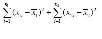
So far, we’ve written residuals as (x_i – x^-). These are represented in Figure 1 as the short horizontal line segments joining each measured value to its respective mean. To indicate the residuals for Sample 1 we’ll add the subscript “1” and write (x_1i – x^-₁); to indicate the residuals for Sample 2 we’ll change the subscript to “2” and write (x_2i – x^-₂). Similarly, the number of replicates for Sample 1 is n₁; the number of replicates for Sample 2 is n₂. We can use this information to form a pooled sum of squares of residuals:

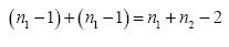
and a pooled degrees of freedom:

Recall that a variance is a sum of squares divided by a degrees of freedom. We’ll create a pooled standard deviation s_p (the square root of a variance) by using our pooled sum of squares of residuals and our pooled degrees of freedom:

The advantage of this pooled standard deviation with four degrees of freedom is that its 95% confidence interval for s_p (based on critical values of the χ²/ν distribution) ranges from 0.60 times its value to 2.87 times its value. The confidence interval from each individual set of replicates based on only two degrees of freedom is broader and ranges from 0.52 times its value to 6.29 times its value. Clearly, the standard deviation is known more precisely with four degrees of freedom than it is with only two. This is essentially why statisticians like big n.

If we’re going to pool more than a few small statistical samples, we need to generalize the notation or the additive numerator in the previous equation is going to go off the page. If J is the number of small statistical samples (J = 2 so far), and if j is an index that refers to a particular small statistical sample (j is either 1 or 2 so far), then we can replace the “+” signs in the previous equation with summation operators (Σ) and form what’s called a “double summation” in the numerator:

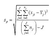
The notation in parentheses in the numerator now uses j to refer to a particular small statistical sample (1 or 2); the same is true for the subscript on n. The denominator first calculates the total number of raw data points that are used and then gives up J degrees of freedom, one for each of the J means that have to be calculated for the J small statistical samples. With this notation, we’re ready for business.

Figure 2 shows the history of a measurement method for which triplicate measurements have been made on 300 physical samples, generating 900 historical data points (J = 300, n₁ = n₂ = Λ = n₃₀₀ = 3). When this information is put into the previous equation to estimate a pooled standard deviation, the number of degrees of freedom is 600. As a result, the 95% confidence interval for s_p now ranges from 0.95 times its value to 1.06 times its value, a very tight interval compared to the intervals for four degrees of freedom (0.60 to 2.87) or two degrees of freedom (0.52 to 6.29). With this many degrees of freedom and this narrow a confidence interval, most statisticians are willing to stretch a bit and call it σ_p, the statistician’s true pooled standard deviation, a so-called population parameter. Let’s say it has a value of 0.8159.

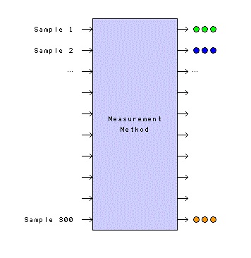Figure 2 – A visualization of a measurement method that has carried out triplicate measurements on 300 physical samples, generating 900 historical data points.

This population parameter is usually given the subscript “m” and is called a (measurement) “method standard deviation,” σ_m. This is a very good estimate of the variability of the measurement method.

Think about what we just did. The method standard deviation is now known very precisely. Is it necessary to carry out more replicates to keep estimating it? If the measurement method behaves in the future as it has behaved in the past, then the answer is “no.” We’ve reached a point of diminishing returns. More replicate measurements will represent an unnecessary cost—they aren’t going to improve our knowledge of σ_m very much. So, let’s save 2/3 of our budget and quit doing replicates on future physical samples that are submitted for analysis, a situation suggested by Figure 3.

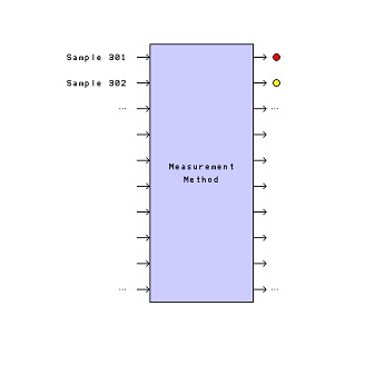Figure 3 – A visualization of the measurement method when σ_m is known and it is no longer necessary to carry out replicate measurements.

If we do this, we can report future values as, for example:

The 95% confidence interval for the true mean will always be the same size: ±1.96 x σ_m = ±1.96 x 0.8159 ≈ ±1.60 about the measured value x (for our example).

There is a slight penalty to be paid for doing this, though. Because of the 1/√n effect, the confidence interval using σ_m and three replicate measurements would be tighter, only 1/√3 = 0.58 as wide. However, if the individual measurements are sufficiently precise for their intended purpose, there is no driving force for doing replicates. If not, it might be cheaper in the long run to redevelop the method to give it a smaller σ_m than to have to average replicates to reduce the uncertainty.

This discussion has assumed homoscedastic noise (see the previous column in this series). If the noise is proportionally heteroscedastic, the analogous equation for the relative standard deviation becomes:

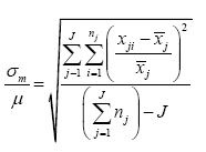
If the measured values are small and get down into the region where homoscedasticity begins to have an effect (remember the Horwitz horn), this equation will “blow up,” so be careful if you use it.

An important assumption about pooling is that the measurement method will behave in the future as it has in the past. I like to check this assumption by running replicates every so often and plotting the results on a control chart. If there is evidence that the variance is increasing, I’ll take measures to find the problem and correct it.

You also need to think deeply about the systems theory diagram for your measurement method. Is it just one method, or is it really an agglomeration of several separate methods? This can be a problem in the pharmaceutical industry where a bioassay is considered to be a single bioassay with its tightly specified SOP. In fact, when more than one bioassayist implements a method, individual differences among bioassayists’ precisions suggest that there is one measurement method for each bioassayist, and any pooling should be done on an individual bioassayist basis. This caution also applies to the construction of control charts—perhaps there should be a control chart for each individual bioassayist. Pooling works best with automated measurement systems for which all unit operations are uniform and consistent with time.

For those of you who don’t feel comfortable giving up those extra replicate measurements, here’s a sobering thought. The next time your physician orders a laboratory test for you, consider the result of that test. It will probably be based on only one measurement. It would be prohibitively expensive to carry out replicate measurements for every laboratory test. Fortunately, most clinical measurement methods have had their σ_m determined during development and the variability of the result (or a surrogate for it) is usually indicated in the lab report the physician receives. If a single measurement is good enough for decisions about your health, maybe a single measurement can be good enough for the decisions you have to make in your work.

I thank Paul Loconto (retired, Michigan Department of Community Health, Bureau of Laboratories) for encouraging a column on pooling, and Stanley Alekman (independent consultant affiliated with Pharmaceutical Advisers, LLC, and The Quantic Group, Ltd.) for helpful insights about pooling, especially when applied to the pharmaceutical industry and to control charts.

Note

Pooling is usually discussed in a more limited way in descriptions of the two-sample Student’s t test or the more general one-way analysis of variance (ANOVA). Almost any good introductory statistics book can serve as a reference.

Stanley N. Deming, Ph.D., is an analytical chemist masquerading as a statistician at Statistical Designs, El Paso, Texas, U.S.A.; e-mail: [email protected]; www.statisticaldesigns.com